Fit any curve
Lines and polynomials, one- and two-phase exponential decay and association, growth, power, logarithmic, Michaelis–Menten, Hill, Gaussian, Boltzmann — or type your own equation. Starting values are found for you.
粘贴您的数据,拟合剂量–反应、酶动力学、指数或您自己的方程,并获取每个参数及其标准误差、95%置信区间和拟合优度。
进行 t 检验、带多重比较的方差分析、非参数检验和卡方检验,然后将图形保存为 SVG、PNG 或 PDF。
曲线拟合与统计是一个即用即算的在线计算器:填好数值,结果会随输入实时更新。 拟合剂量–反应(IC50/EC50)、酶动力学、指数和自定义方程。
在对应字段填入数字,例如金额、利率、身高体重或日期。
切换货币、单位或计算模式,工具会自动按所选口径换算。
结果区会实时显示答案,通常还会给出分步过程或明细。
点击复制按钮把结果带走,也可截图保存或清空重算。
Lines and polynomials, one- and two-phase exponential decay and association, growth, power, logarithmic, Michaelis–Menten, Hill, Gaussian, Boltzmann — or type your own equation. Starting values are found for you.
Four- and five-parameter logistic fits give the IC50/EC50 with its confidence interval. Type unknown Y values to read concentrations off a standard curve.
Standard errors and 95% confidence intervals of every parameter, R², adjusted R², Sy.x, RMSE, AICc, the runs test and a residual plot. Compare two equations by F test and AICc.
Unpaired, Welch and paired t tests, Mann–Whitney and Wilcoxon, one-way ANOVA with Tukey, Bonferroni or Dunnett, Kruskal–Wallis with Dunn, and two-way ANOVA. Also from mean, SD and N.
Descriptive statistics, Shapiro–Wilk and D’Agostino normality tests, Grubbs’ outlier test, Pearson and Spearman correlation, chi-square and Fisher’s exact test with odds ratio and relative risk.
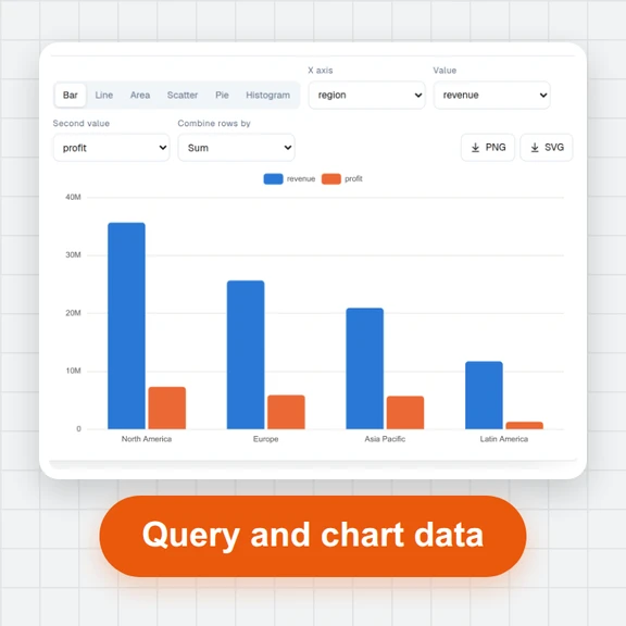
Scatter with fitted curves and confidence bands, bar, dot, box and violin plots, error bars, significance brackets, log axes. Vector SVG and PDF with embedded fonts, PNG at print resolution.
Dose–response equations use log(dose) as X. If your X column holds concentrations, tick “X values are concentrations” — points at zero concentration are left out.
If the response must start at 0 or end at 100%, open Constraints and fix Bottom or Top. Fewer free parameters give tighter confidence intervals.
For paired t and Wilcoxon tests, keep each subject’s two values on the same row of the Column table.
SD shows how spread the values are; SEM how precisely the mean is known. Say which one your error bars show in the legend of your figure.
Copy puts the result tables on the clipboard ready to paste into a spreadsheet or document; CSV saves them as a file.
Write Y = Bottom + (Top − Bottom)/(1 + exp((V50 − x)/Slope)). Any name other than x becomes a parameter; log is base 10, ln is natural.
无需注册即可试用,游客每日 3 次免费。所有处理都在你的设备上完成,文件不会被上传。
所有工具每天都有免费额度。 游客每日 3 次免费,注册再送 20 积分。文件不上传,处理全在你的设备上完成。
是的。无需账户,图表没有水印,拟合或测试没有限制,也没有付费等级。
不。每个计算都在你的浏览器标签中运行。页面只下载用于绘制图形文本的开放字体;你的数值从未被发送到任何地方。项目只保存在这个浏览器中。
拟合引擎能够重现所有27个NIST StRD非线性回归参考问题的认证值——采用NIST的第二组初始值,最佳拟合参数至少精确到6位有效数字。使用NIST的第一组有意不良的初始值时,两个最难的问题(BoxBOD和MGH10)会停在不同的极小值上,这在大多数拟合程序中也是如此。每一次测试和拟合也都会与广泛使用的开源科学库进行对比检查。
将 log(浓度) 放在 X 列(或者直接放浓度,并勾选“X 值为浓度”),将反应放在 Y 列,并选择“log(剂量) 对反应,4 参数”。结果显示 LogEC50 以及带有 95% 置信区间的 EC50/IC50。对于抑制曲线,Hill 倾斜度为负。
描述性统计;非配对、Welch 和配对 t 检验;单样本 t 检验和 Wilcoxon 检验;Mann–Whitney 检验;Wilcoxon 配对检验;单因素方差分析带 Tukey、Bonferroni 或 Dunnett 事后检验,Welch 方差分析,Bartlett 和 Brown–Forsythe 检验;Kruskal–Wallis 检验带 Dunn 事后检验;双因素方差分析带行内比较;Pearson 和 Spearman 相关;卡方检验和 Fisher 精确检验;Shapiro–Wilk 和 D’Agostino–Pearson 正态性检验;Grubbs 异常值检验。
是的。在你的电子表格中选择单元格,复制,然后点击表格中的一个单元格并按 Ctrl+V(在 Mac 上为 Cmd+V)。小数逗号是可以识别的。你也可以导入 CSV、TSV 和 .xlsx 文件。
它没有重复测量方差分析,没有跨数据集共享参数的全局拟合,Fisher 精确检验仅适用于 2×2 表,没有 ROUT 离群值方法,也没有生存分析。双因素方差分析需要单个重复值。非常大的 Dunnett 比较(数十个组)只需几秒钟。
无(普通最小二乘法)、使用每个点的 Y 值的相对 1/Y²,或使用每个 X 的重复测量的标准差或你的标准差列的 1/SD²。加权拟合报告加权平方和和 R²。
SVG and PDF are vector files: lines and text stay sharp at any size, and the PDF embeds its fonts. PNG goes up to 1200 dpi and records its resolution. Fonts have the same widths as Arial and Times New Roman.
粘贴数值,选择一个方程或测试,然后导出图表。